Crabs All the Way Down: Running Rust on Logic Gates

A journey in building an ARM CPU from scratch in a digital circuit simulator, and running Rust on it to interpret Scheme and serve Web pages.

Posted Aug 17, 2022 Updated Dec 3, 2024

By zdimension

27 min read

This article will discuss many topics, from CPU architecture design to historical shenanigans. Take a drink, it’s downhill from there.

Even though the number has steadily decreased since the 90s, there are still many different and incompatible CPU architectures in use nowadays. Most computers use x86_64 and pretty much all mobile devices and recent Macs use some kind of ARM64-based ISA (instruction set architecture).

In specific fields, though, there are more exotic ones: most routers still use MIPS (for historical reasons), a roomful of developers use RISC-V, the PS3 used PowerPC, some servers 20 years ago used Itanium, and of course IBM still sells their S/390-based mainframes (now rebranded as z/Architecture). The embedded world has even more: AVR (used in Arduino), SuperH (Saturn, Dreamcast, Casio 9860 calculators), and the venerable 8051, an Intel chip from 1980 which is still being produced, sold and even extended by third parties.

All these architectures differ on their defining characteristics, the main ones being:

word size: 8, 16, 31, 32, 64 bits, sometimes more
design style: RISC (few instructions, simple operations), CISC (many instructions, performing complex operations, VLIW (long instructions, doing many things at once in parallel)
memory architecture: Harvard (separate code memory and data memory), von Neumann (shared)
licensing costs: RISC-V is open and free to use, whereas x86 and ARM, for example, require licensing fees
broadly, their feature set: floating-point numbers (x87), encryption (AES-NI), support for native high-level bytecode execution (Jazelle, AVR32B), vectorized computation (SSE, AVX, AltiVec)

That’s not even counting DSP architectures, which are, to put it lightly, the ISA counterpart to the Twilight Zone (supporting weird arithmetic operations, peculiar data sizes, etc).

A lot of people have built homemade CPUs, either on real breadboards or in software, for emulators or circuit synthesis. It’s a very interesting project to do, even for beginners (really, check out Ben Eater’s video series), because it really helps grasp how code translates to the electrical signals that power every device we use, and how complex language features can really be implemented on top of simple operations.

Making a CPU

A number of circumstances have led me to design a simple ARM-ish CPU in a digital circuit simulator. I originally used logisim-evolution (of which I have since become a member of the development team), and recently migrated the circuit to Digital, for performance reasons (Logisim couldn’t simulate my circuit at more than 50 or 60 Hz, whereas Digital reaches 20 kHz).

ARM, because it supports a subset of the ARM Thumb instruction set, which itself is one of the multiple instruction sets supported by ARM CPUs. It uses 32-bit words, but the instruction are 16 bits wide.

-ish, because, well, it only supports a subset of it (big, but nowhere near complete), and is deliberately limited in some aspects. Weird instructions, such as the PUSH / POP / LDM / STM family (one of the big CISC ink blots in the RISC ARM ISA), are not supported and are implemented as manual load/stores by the assembler. Interrupts are not supported either.

Pedantically, I didn’t design only a CPU but what one could call a computer; it has a ROM, a RAM, and various devices that serve as the “front panel”.

Quick sidenote: devices

To be really useful, a computer will not only have a CPU and a memory chip. It’ll also have peripherals and other items plugged into it: a keyboard, a screen, a disk drive, speakers, a network card; pretty much anything you can (or can’t) imagine has already been made into a computer device.

At the end of the day, the only thing you need is to be able to transmit data to and from the device. There are two opposite ways to do this: either devices are ✨special✨, either they aren’t.

Basically, some architectures (x86, I’m looking at you) have, in addition to the memory, a special, separate address space for I/O, with its own special, different instructions: on an 8086, you’d use MOV to read and write main memory, and IN / OUT to read and write to a device. Some devices (the most important ones: PS/2 controller, floppy disk, serial port, …) have a fixed port number, other have a port number assigned at boot by the BIOS. In the olden days, it was common practice to require setting environment variables or writing config files to inform software of which devices were plugged were (e.g. the famous BLASTER config line). This is called PMIO (port-mapped input/output).

The other option, the one used by pretty much everybody else, including modern x86 computers, is to have a single unified address space, but to make it virtual.

I’m using the word virtual here to differentiate this unified address space from the real physical memory address space (which, in itself, only really means anything on machines with a single memory unit). There’s another concept called virtual memory that designates a completely unrelated (though similar in fashion) thing: providing programs with an address space larger than the computer’s RAM through the use of strategies like swapping that allow moving RAM pages to the disk storage to free space in the working memory, and most importantly isolating programs running on the same computer.

Imagine how IP addresses are supposed to map the entire Internet, but in reality an address does not have to exactly map to a single machine somewhere. For example, 127.0.0.1 (::1 in IPv6) is the local loopback, and maps to the machine you’re using. This is not required to be known by software communicating over the network, since the mapping is done by the network stack of the OS.

It’s the same here: areas of the (virtual) address space are mapped to physical components. To give you a real-world example, here’s the NES’s address space:

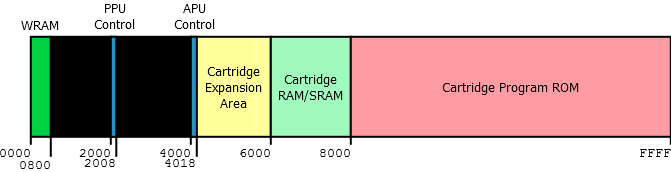
image from https://jarrettbillingsley.github.io/

How to read: addresses from 0 to 800 (hexadecimal) are mapped to WRAM (work RAM), from 2000 to 2008 to the PPU (graphics card) control registers, from 4000 to 4018 to the APU (sound card), I trust you can take it from there. This is called MMIO (memory-mapped input/output).

The big advantage of this approach, for me, is really its simplicity, CPU-wise: it’s just memory! Take the address of the device’s area, read, write, it’s really simple. It also makes things easier software-wise: you don’t have to write inline assembly to call special instructions; as long as you can read and write from pointers, you’re good to go.

In addition to this, memory mapping can also be used to provide access to different memory chips (e.g. ROM and RAM). Here’s what it looks like for my circuit:

Notice the arrows on each side of the edges between the components and the mapper; they indicate whether the component is read-only, read/write or write-only.

The CPU

It’s simple, really. I mean, compared to real CPUs.

As in real Thumb, there are sixteen 32-bit registers, numbered r0 through r15. The last three have nicknames: r13 is sp (stack pointer), r14 is lr (link register) and r15 is pc (program counter).

Quick sidenote: stack pointer

Memory is hard. I’ll talk about it later.

16 is a lot; so in reality they’re divided into the low (r0-r7) and high (r8-r15) registers. High registers can only be manipulated using specific instructions, so the low ones are the ones you’re gonna use in everyday life.

Instructions are grouped into several categories, each containing instructions with a common header. I won’t list them all here, but the most used ones are the ALU (arithmetic and logic) operations, the load/store instructions (relative to pc, to sp, or to a general register), the stack manipulation instructions and the branch instructions (conditional and unconditional).

Instruction groups are handled by separate, independent subcircuits, that all write into shared buses.

Quick sidenote: buses

Bus is a surprisingly polysemic word. It has definitions in more domains than I can count, and even in electronics and hardware it’s used for a variety of things. The common factor between all those definitions is “thing that links other things”.
As in previous parts, I will be simplifying the explanation anyway, because electronics is a vast field of study.

In circuit design parlance, a bus is a group of wires connected together. Specifically, in this case, it’s a group of wires where only one wire emits a signal at a given instant. Electrically, this is permitted by the use of what’s called tri-state logic: a signal is either 0, 1 or Z (pronounced “high-impedance”). Z is “weak”, in the sense that if you connect a Z signal with a 0 or 1 signal, the output will be that of the second signal. This is useful: you can have lots of independent components, each with an “enable” input, that only output a signal if they are enabled, and otherwise output Z. The basic component used for this is called, fittingly, a tri-state buffer. It’s a simple logic gate that, if enabled, outputs its input unchanged, and otherwise outputs Z.

All these components can then be plugged together, and you can enable one and get its output easily.

Component example: load/store with register offset

This is the component that handles instructions of the form {direction}R{sign}{mode} {destination}, [{base}, {offset}], with:

{direction}: either LD (load) or ST (store)
{sign}: either nothing (do not extend), or S (sign-extend the value to fill 32 bits)
{mode}: either nothing (full word, 32 bits), H (halfword, 16 bits) or B (byte, 8 bits)
{destination}: the target register, to read from/write to
{base}, {offset}: the address in memory (which will be the sum of the values of both)

As an example, ldrh r1, [r2, r3] is roughly equivalent to r1 = *(short*)(r2 + r3) in C code.

The instructions for this group are encoded as follows:

15	14	13	12	11	10	9	8	7	6	5	4	3	2	1	0
0	1	0	1	opcode			Ro			Rb			Rd

opcode is a 3-bit value encoding both {direction}, {sign} and {mode}.

{direction} has two possible values (load, store); {sign} has two (raw, sign-extended) and {mode} has three (word, halfword, byte). That’s 2⋅2⋅3 = 12 possible combinations, more than the 23 = 8 possible values for opcode, which means that some combinations are not possible.
This is because only load operations for incomplete (halfword, byte) values can be sign-extended, so the invalid combinations (strsh, strsb, strs, ldrs) are not given an encoding.

Here’s the circuit:

Here are the different exotic logic components used here:

the small triangles are tunnels: named wires that are accessible anywhere in the circuit;
the big trapezoids are multiplexers: they output the nth input, where n is also an input;
the three-wired triangles are buffers: they output their input if the side wire is high, otherwise they output Z (high-impedance);
the yellow boxes convert a 3-bit low register number into a 4-bit register number (by adding a zero in front of it);
the large rectangles with integer ranges next to them are splitters: they split a multi-bit value into multiple smaller values, to access individual bits or bit ranges

From top to bottom:

the three registers (Rd, Rb, Ro) are read from the instruction at their respective positions (0-2, 3-5, 6-8) and sent to the corresponding global tunnels (RW, RA, RB)
opcode is decoded to check whether it’s a store (000, 001, 010) or a load (remaining values)
opcode is decoded to find the value of mode: 0 for word, 1 for halfword, 2 for byte
opcode is yet again decoded to find the value of sign (true only for opcodes 011 and 111 so we can check that the last two bits are high)

The Instr0708 tunnel is the activation pin for this component; it’s high if the current instruction belongs to this instruction group.

Pretty much all other components look like this one, and when you plug them all together, you get a circuit that can execute instructions.

Quick sidenote: memory is hard

The seemingly simple problem of manipulating data and storing it somewhere so that you can get it back later is actually… not simple. Giving your CPU access to a big linear array of memory cells is not enough, you have to decide what you are going to do with it. Look at this Python program:

        
      
print("Hello, World!")

Where should the string be stored? It’s gotta be somewhere. What about print? It’s not an instruction, it’s just a global variable that happens to be set to an object of type builtin_function_or_method, that you can call with the () operator. It’s gotta be stored somewhere too. Remember, the only thing you really have at the moment is a big array of numbers. On top of that, the only set of operations you really have is {"load value from address", "store value at address"}. Or is it?

The CPU speaks in assembly instructions. These instructions have a fixed, defined encoding, and on the ARM Thumb instruction set they always (i.e. almost always) have the same size: 16 bits. Ignoring the header of the instruction (that tells you which one it is), that will take up a few bits, we quickly see that if we were to give address as immediates (constant values, in the instruction), we couldn’t address more than 216 bytes of memory.

Hence: addressing modes and memory alignment.

If we look at everyday life programs, we can observe that there are two main use cases for memory: storing local variables (variables in functions, or parameters), and storing global variables (global configuration, memory that will be shared between programs).

Use case	Allocation size	Maximum lifetime	Time of allocation	Time of free
Local	Generally small	Current function call	When entering function	When leaving function
Global	Any	Static (lifetime of the program)	Any	Any

There’s a clear difference: on one hand, “local memory”, which is used for small, deterministic allocations, and “global memory”, which is used for anything, at any time, with very few constraints.

How does that map to our “big block of cells”? We’ll start with the “global” memory. We don’t really know anything about how it’ll be used, so we can’t make too many assumptions. You can ask for any amount of bytes at any moment, and give it back to the OS any time you want, and you usually expect “given-back” space to be useable by subsequent allocations. This is hard. The real-world equivalent would be a big pile of stuff, laying on the ground, waiting for some program to pick it up, use it, or throw it in the trash. For this reason, it’s called the heap.

Next, we can see that the “local memory” evolves in a specific way: it grows when we enter a function, shrinks when we exit it, and function calls follow a stack-like pattern (when you’ve entered a function, you can do anything you want, but you always end up exiting it at some point). In fact, it really is a stack (in the algorithmic data structure meaning); it’s got two operations: push (grow) and pop (shrink). This “local memory” is called the stack.

Since it grows and shrinks that way, we don’t really have to do any bookkeeping of the blocks of allocated memory, where they are, what strategy to use to choose where to allocate new blocks, etc. The only piece of data we need is the “depth” (i.e. how deep we are in that stack, or in other words, the length of the stack). The way this is usually done is that we set some place in memory to be the beginning of the stack, and we keep a global variable somewhere (for example, in a register) that contains the position in memory of the topmost item of the stack: the stack pointer (on ARM, sp, or its full name r13).

There’s something I haven’t specified yet: which direction the stack grows. Some architectures make it grow upward (push = increment stack pointer, pop = decrement), but most do it the opposite way and make it grow downward. Growing it downward means that you can easily make the heap start at address 0 and make the stack start at whatever the maximum address is, and you’re assured that they won’t collide until the heap grows too far up or the stack grows too far down.

In memory parlance, upward means increasing and downward means decreasing. “The stack grows downward” means that growing the stack decreases the stack pointer, and vice versa. Many diagrams online illustrate memory with the address 0 at the top, suggesting that downward means increasing, but this is misleading.

Now that we know how memory works, how do we access it? We’ve seen that we can’t address it all, since instructions are too small, so how can we counter that?

Well, the answer is to use different addressing modes. For example, if you want to access memory on the stack, you’ll usually be accessing things that are on top of the stack (e.g. your local variables), so instead of giving the full memory address (big), you only have to give the distance to the data relative to the stack pointer (small). This is the sp-relative addressing mode, and looks like ldr r1, [sp, #8].

Additionally, we can assume you will mostly store things that are 4 bytes or bigger, so we’ll say that the stack is word-aligned: everything will be moved around so that addresses are multiples of 4. This means that we can fit even bigger numbers in the instruction: we only have to store the offset, divided by 4. The instruction above would encode its operand as 2, for example.

Sometimes, you’ll want to store data that is only useful to a single function. For example, switch / match instructions are usually implemented using jump tables: a list of offsets is stored in the program, and the correct offset is loaded and jumped to. Since this will be stored in the code of the function itself, it becomes useful to perform memory operations relative to the current position in the code, and that’s how get get pc-relative addressing: ldr r2, [pc, #16]. As with sp, memory is word-aligned, so the offset has to be a multiple of 4.

Quick sidenode: function calls

The simplest way to call functions, in assembly, is through the use of jumps. You put a label somewhere, you jump to it. There’s a problem though: how do you go back? A function can be called from multiple places, so you need to be able to “remember” where the function was called from, and you need to be able to jump to an address, rather than to a known label.

The simple approach, like with the stack pointer before, is to use a global variable (i.e. register) to store the address of the caller, and to have a special jump instruction that sets the register to the current position (linking), so we can go back to it later (branching). On ARM, this is the bl (branch-link) family of instructions, and that register is called the link register (abbreviated lr, nickname of r14).

But there’s another problem: it doesn’t work for nested calls! If you call a function from inside another called function, the value of the link register gets overwritten.

This is actually not a new problem: other registers can get overwritten as well when you call a function, and you can’t expect the programmer to read the code of every function they’re calling to see which registers are safe and which aren’t. Here comes the calling convention: on every architecture (x86, ARM, …) there’s a set of rules (the ABI) that tell you how everything works, what a function is allowed to do, and specifically what registers should be preserved by the callee. A preserved register is not read-only: the callee can do whatever it wants with it, as long as when the control is given back to the caller, the old value is back.

The way to solve this is through register saving. When entering a function, space is allocated on the stack for local variables but also for registers that have to be preserved, and when exiting, the original values are pulled back from the stack into the registers.

Among those registers, on ARM, the link register is saved too. One cool aspect of ARM special registers being useable as general-purpose registers, is that you don’t have to use a branch instruction to jump somewhere: you can just write into pc!

The usual pattern for functions in ARM assembly is thus:

        
      
my_function:
    push {r4, r5, lr} ; save r4, r5 and lr
    movs r4, #123 ; do stuff
    movs r5, #42
    pop {r4, r5, pc} ; restore the values to r4, r5 and *pc*!

Devices

Not much is needed to make a circuit look like a computer. For starters, you may want to start with:

a keyboard (reading raw character input);
a terminal display (displaying characters, like a terminal emulator);
a video display (displaying raw pixel data);
a random number generator;
a decimal 7-segment display;
a network card (that can receive and transmit data via TCP).

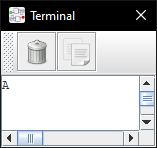
All of these are seen as addresses in memory by the CPU and programs running on it. For example, writing a byte to address 0xFFFFFF00 will display a character in the terminal display. Reading a byte from address 0xFFFFFF18 will tell whether the keyboard buffer is empty or not.

Running code

The simplest way to run code on this thing is to simply write machine code and load it into the ROM.

Here’s a simple program:

        
      
movs r0, #255	; r0 = 255 (0x000000FF)
mvns r0, r0		; r0 = ~r0 (0xFFFFFF00, address of terminal)
movs r1, #65    ; r1 = 65  (ASCII code of 'A')
str r1, [r0]    ; *r0 = r1

It’s assembled as 20ff 43c0 2141 6001 (8 bytes), and when loaded and run, it shows this after 4 cycles:

Of course, writing programs in assembly isn’t exactly practical. We invented macro assemblers and high-level (compared to assembly) programming languages for this a long time ago, so let’s do that here. I originally went with C, but quickly switched to Rust for the ease of use and powerful macro support (useful for a constrained environment like this one).

Rust (technically, the reference compiler, rustc) uses LLVM as a backend for compilation, so any target LLVM supports, Rust supports it to some extent. Here, I’m using the builtin target thumbv6m-none-eabi (ARM v6-M Thumb, no vendor or OS, embedded ABI), but there’s a big constraint: my CPU is not a full ARM CPU.

Since not all instructions are supported (some are emulated by my homemade assembler), I can’t just build ARM binaries and load them. I need to use my own assembler, so I’m calling the compiler directly and telling it to emit raw assembly code, which is then sent to my assembler that finally generates a loadable binary file.

Additionally, since I’m running code without an OS, without any external code, I can’t use Rust’s standard library. This is a perfectly supported use case (called no_std), and doesn’t mean I can’t use anything at all: it only means that instead of using the std crate (the usual standard library), I use the core crate that contains only the bare necessities and specifically does not depend on an operating system running underneath. The core crate however does not include anything that relies on heap allocations (such as String or Vec), these are found in the alloc crate that I don’t use either for a number of complex reasons related to my build system.

Basically, I wrote my own standard library. I’m now able to write programs like:

        
      
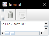
fn main() {
    println!("Hello, world!");

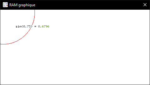
    screen::circle(10, 10, 20, ColorSimple::Red);

    let x = fp32::from(0.75);
    let mut video = screen::tty::blank().offset(50, 50);
    println!("sin(", Blue.fg(), x, Black.fg(), ") = ", Green.fg(), x.sin(), => &mut video);
}

and get:

Pitfalls

Using rustc’s raw assembly output means that I can’t rely on code from other crates than the one I’m building (that would require using the linker, which I am not using here). I can’t even use the compiler’s intrinsics: functions such as memcpy or memclr are often used to perform block copies, but they aren’t present in the generated assembly, so I had to implement them myself (I borrowed some code from Redox here).

Another problem is that since I am emulating some instructions (by translating them into sequence of other, supported instructions), branch offsets can get bigger than what the compiler expected. Problem: conditional branches on Thumb take an 8-bit signed immediate, so if you try to jump more than 128 instructions ahead or behind, you can’t encode that instruction.

In practice, this means that I often have to extract code blocks from functions to make them smaller, and that the whole codebase is sprinkled with #[inline(never)] to force the compiler to keep these blocks in separate functions.

Implementing a useable standard library is not the easiest task; ensuring that the whole thing is ergonomic and pleasant to use is even harder. I had to use many unstable (nightly-only) features, such as GATs, associated type defaults, and specializations, among others.

This whole project comforts my choice to use Rust for future low-level/embedded development projects. Doing a hundredth of this in C would have been orders of magnitude harder and the code wouldn’t have been anywhere as readable as this one is.

Showcase

Plotter

This plotter uses the fixed-point (16.16) numeric library and the video display.

Trigonometric functions were implemented using Taylor series (I know, CORDIC, but I like pain).

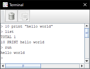
BASIC interpreter

This is a simple BASIC interpreter / REPL, similar to what was found on home computers of the 80s (e.g. C64). You can input programs line by line, display them, and run them. The supported instructions are PRINT, INPUT, CLS, GOTO and LET. The prompt supports LIST, RUN, LOAD, ASM and ASMRUN.

“Hello World” program

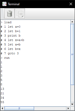
Programs can also be loaded over the network (similar to cassette loading on the C64), with a program such as:

        
      
cat $1 <(echo) |	# read file, add newline
dos2unix |			# convert line ends to Unix (LF)
nc -N ::1 4567		# send to port

Here, LOAD starts listening and the received lines are displayed with a # prefix and read as if they were being typed by the user:

Fibonacci sequence, loaded over network

Programs can also be compiled to Thumb assembly for higher performance:

In case you’re wondering, here’s how that part works:

each BASIC instruction and expression is converted (compiled) to a sequence of assembly instructions, for example CLS simply stores 12 (\f) in the address of the terminal output, while an expression simply sets up a little stack machine that evaluates the formula and stores the result in r1, and a LET instruction evaluates its expression and stores r1 into the variable’s memory cell
once the program has been compiled, it’s executed like a function, like this:

        
      
let ptr = instructions.as_ptr();
let as_fn: extern "C" fn() -> () = unsafe { core::mem::transmute(ptr) };
as_fn();

a bx lr instruction is appended at the end of the instruction list, so when the program finishes, it gives the control back to the interpreter

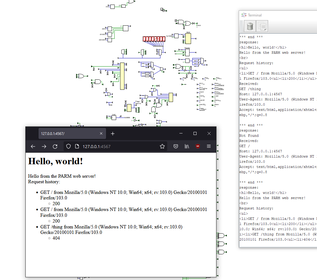
Web server

This program listens for HTTP requests, parses them, and processes them.

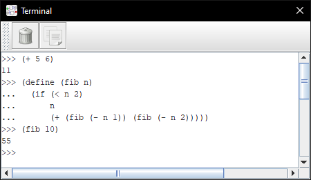
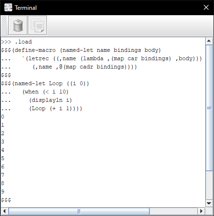
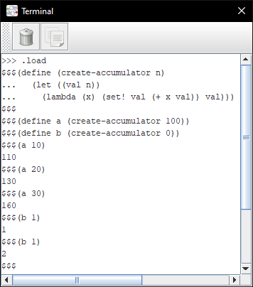
Scheme

This is an REPL for a small but useable enough subset of R6RS. It supports most important primitive forms, many builtins and macros.

Supported datatypes are symbols, integers, booleans, strings, lists (internally stored as vectors), void and procedures (either builtin functions or user-defined closures).

addition and Fibonacci sequence

As with the BASIC interpreter, programs can be loaded over the network:

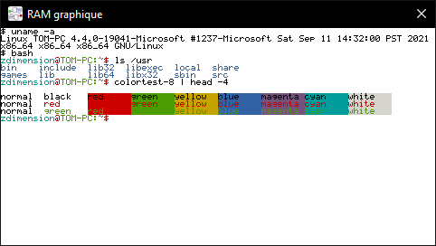
macro creating the named-let form, allowing for easier loop definition

function that creates a mutable accumulator, using closures

Terminal emulator

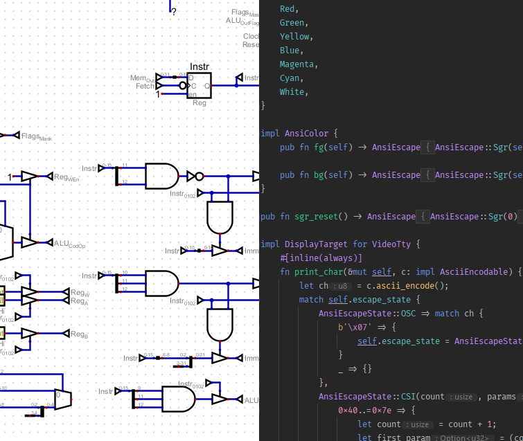
This is a simple terminal emulator that supports a subset of the ANSI (VT) escape codes (enough to display pretty colors and move the cursor around).

It uses a 5x7 font borrowed from here, and the ANSI decoding logic was written by hand (there are crates out there that do just that, but they support all the ANSI codes, whereas I only needed a very small subset for this program).

A script such as this one can be used to start a shell and pipe it to the circuit:

        
      
exec 3<>/dev/tcp/127.0.0.1/4567
cd ~
unbuffer -p sh -c 'stty echo -onlcr cols 80 rows 30 erase ^H;sh' <&3 1>&3 2>&3

MIDI player

Digital provides a MIDI output component, that supports pressing or releasing a key for a given instrument, so I wrote a simple program that uses midly to parse a MIDI file sent over network and then decodes useful messages to play the song.

Since channels are stored sequentially in a MIDI file, and since I only have one output anyway, I wrote an algorithm that merges channels together into a single message list. Events are already stored chronologically, so this is simply a “merge k sorted arrays” problem, that can be solved by recursively merging halves of the array (traditional divide-and-conquer approach) in $O(n k \log k)$ ($k$ arrays of $n$ items).

Here’s the result:

Parting words

All in all, this was fun. ARM/Thumb is a good architecture to implement as a side project, since it’s well-supported by compilers and a small enough subset of it can suffice to run interesting code. Logisim and Digital are both excellent tools for digital circuit simulation. Rust is nice for doing things and making stuff.

Repository available here. Don’t look at the commit messages.

Long posts

Programming Hardware Rust

This post is licensed under CC BY 4.0 by the author.