Stack Machines and Where To Find Them

Ever tried googling “recursion”?

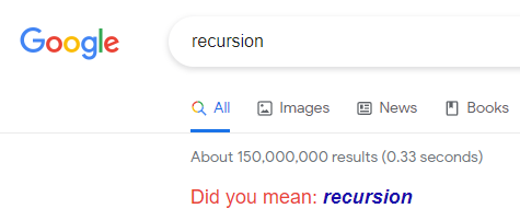
There’s something quite peculiar about recursion. Every developer and their dog has heard of it at some point, and most developers seem to have quite a strong opinion about it.

Sometimes, they were taught about it in college. Some old professor with a gray beard and funny words (the hell’s a cons cell? why are you asking if I want to have s-expr with you?) made them write Lisp or Caml for a semester, growling at the slightest sign of loops or mutability to the poor student whose only experience with programming yet was Java-like OOP. Months spent writing factorials, linked lists, Fibonacci sequences, depth-first searches, and other algorithms with no real-world use whatsoever.

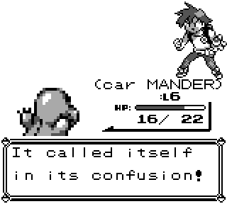
Other times, it was by misfortune. While writing code in any of their usual C-family enterprise-grade languages, they accidentally made a function call itself, and got greeted by a cryptic error message about something flowing over a stack. They looked it up on Google (or Yahoo? AltaVista? comp.lang.java?) and quickly learned that they had just stumbled upon some sort of arcane magic that, in addition to being a simply inefficient way of doing things was way too complicated for any practical developer to understand.

---

Disclaimer: this is a long post. We’ll first see what recursion is about and why you should use it. Then, we’ll see how functions work (down under; buckle up we’re gonna write assembly code and Fortran), invent automatic memory, and see why you shouldn’t use recursion.

We’ll take a quick detour in optimization land to explain why you should use recursion sometimes, and have a little theoretical trip to really understand what’s under recursion, and why some things are inherently recursive and others aren’t.

We’ll have a language stay and learn a bit of Polish (notation), and discover the power of stack machines. To conclude, we’ll try writing a Rust macro that parses and executes Forth code at compile time.

---

WYSIWYG

I’m gonna use multiple programming languages in this post, because I want to make it clear that all of this is not specific to one language in particular. The logic itself is what matters.

Programs, algorithms in general, tend to follow the structure of the data they process.

If all you’ve got is an array, most things you’ll want to do will be linear processing of that array. Computing a sum, displaying each element, any sort of linear tasks. And the programs implementing these tasks will mostly have the same structure:

for elem in list:
	action
    
# sum
accum = 0
for elem in list:
	accum += elem
    
# display
for elem in list:
	print(elem)

Usual imperative, iterative code. I used arrays as an example here, but strings would have worked just as well. But loops only get you so far.

Let’s say we’re not working with arrays anymore, we want to perform various tasks on the file system. Imagine your C: drive, or your root file system (/). Everything in your file system is either a file, or a directory that can contain other things.

type fs_item =
	| File of { name : string }
	| Directory of { name : string; contents : fs_item list }

We immediately see the fs_item type is recursive; a directory can contain a list of fs_items.

Let’s say we want to get the total number of files in a directory. By total, I mean count files in subfolders, etc. We need to start from the directory we want to analyze, count its files, and then… for each of its subdirectories, do the exact same. Count the files, analyze the subdirectories, count their files, analyze their subdirectories.

fn count_files(item: &FsItem) -> int {
    match item {
        File { .. } => 1,
        Directory { contents } => {
            let mut count = 0;
            for item in contents {
                count += count_files(item);
            }
            count
        }
    }
}

We’ve got ourselves a recursive function. It’s readable, too. If you look at the code, you’ll see it follows the exact same structure as our “ideal” algorithm we wrote earlier.

Now, sure, this can be done iteratively. With a stack:

fn count_files(item: &fs_item) -> int {
    let mut stack = vec![item];
    let mut count = 0;
    while let Some(item) = stack.pop() {
        match item {
            File { .. } => count += 1,
            Directory { contents } => stack.extend(contents),
        }
    }
    count
}

It’s immediately a lot less obvious what the code does. At first glance, we’re creating a list, that we’re… popping an item from? Then we extend the list? It just doesn’t directly evoke counting files in a directory.

This is one example of a general algorithm where recursion shines compared to iteration. It’s called the depth-first search, and it’s useful in a lot of contexts. Everywhere you have a tree structure, basically. Some examples of tree structures in everyday life:

• the file system (files & directories)
• a syntax tree (code blocks, expressions): easy cases are XML, HTML and JSON
• employee hierarchy (employees and managers)
• scene graph (entities, sub-entities with matrices, etc)

Coming back to the code, these two implementations are really equivalent: the recursive one also uses a stack… but it’s hidden.

We’ll see later that the opposite is also true: the iterative one also uses recursion…

---

Functions from Scratch (any%)

The CPU in your computer is really simple, from the outside. It’s a magic box that reads instruction X, processes it, moves stuff around and goes on to read instruction X+1. It doesn’t know nor care about fancy high-level concepts such as “functions” or “types”. It manipulates registers and memory cells, both of which containing fixed-size integers, and each instruction is independent from the others.

Well, sometimes, it doesn’t go on to read instruction X+1. Sometimes, instruction X is something called a “jump”, or “branch”, that tells the CPU to instead go find instruction Y, which can be anywhere specified by the instruction. It can be “jump ahead 5 instructions” or “jump directly at address 18236”. This allows for things like an if-statement:

1	set reg0 = 5
2	set reg1 = 8
3	set reg2 = 0
4	compare reg0, reg1
5	if greater than, jump to 7
6	set reg2 = 1
7	display reg2		<-- contains 1 iff reg0 <= reg1

Great, we’ve got conditionals (and loops). Maybe we can get functions, too?

1	set reg0 = 5
2	jump to SQUARE
3	display reg0
4	end

SQUARE:
5	set reg0 = reg0 * reg0
6	go... back?

Entering the function is simple, we just have to jump to its first instruction. But how do we return? How do we go back where we jumped from? We’d need to somehow save the instruction where we want the function to return to, so it can jump to it when it’s finished. Something like this:

1	set reg0 = 5
2	set ret_addr = 4
3	jump to SQUARE (6)
4	display reg0
5	end

SQUARE:
6	set reg0 = reg0 * reg0
7	jump to address in ret_addr

And it works! We use a special kind of register that’s used specifically for storing the return address, and we just have to jump to it when the function’s finished. However, what happens if we call a function from inside a function?

---

Nested calls

1	set reg0 = 5
2	set ret_addr = 4
3	jump to SQUARE_PLUS_ONE (8)
4	display reg0
5	end

SQUARE:
6	set reg0 = reg0 * reg0
7	jump to address in ret_addr

SQUARE_PLUS_ONE:
8	set ret_addr = 10
9	jump to SQUARE (6)
10	set reg0 = reg0 + 1
11	jump to address in ret_addr

Did you spot the issue?

SQUARE_PLUS_ONE overwrites ret_addr so that it can call SQUARE, so the original value is lost. When it tries to return to its caller (to end up at line 4), it instead goes back to line 10, and it goes in an infinite loop.

There’s an easy solution: make each function have its own ret_addr register. You’ll have ret_addr_SQUARE, ret_addr_SQUARE_PLUS_ONE, etc. When you call function F, you set ret_addr_F and you jump to F.

Problem solved. You can call functions, and they themselves can call other functions.

This is how FORTRAN handled subroutines (old-timey name for functions) in the olden days of UPPERCASE PROGRAMMING. Each function in the program had a static, fixed, compile-time known zone in the memory that stored its local variables and the return address. When you called a function, it would initialize that area, alongside the return address.

Here’s an example (lowercased) program exhibiting this behavior:

program main
	! Since Fortran prohibits recursion by default,
    ! I'm tricking the compiler by passing a reference
    ! to the function, so it doesn't know it's calling
    ! itself.
    call count(5, count)

    contains
    subroutine count(i, ref_to_count)
        integer :: i, temp
        external ref_to_count

        temp = i * 2 ! assign a value to temp
        if (i > 1) then 
            call ref_to_count(i - 1, ref_to_count) ! recursion
        end if
        print *, temp ! print the value we assigned before
    end subroutine
end program

Here’s what the program prints:

2
2
2
2
2

Since the function cannot call itself, the compiler knows there aren’t ever “two calls of the function at the same time”. The local variables are thus allocated statically, i.e. in the global space. But here, we’re tricking the compiler into letting us call count recursively, so we’re encountering an important problem: inner function calls overwrite locals from the outer one. Obviously, since the locals are… global.

We can actually get the same behavior in C by forcing the local variable temp to be allocated statically: (we’ll see later in detail what this means)

void count(int i) {
    static int temp;
    temp = i * 2;
    if (i > 1) {
        count(i - 1);
    }
    printf("%d\n", temp);
}

int main() {
    count(5); // will print "2" five times
}

In Fortran, if we make the function recursive, the problem doesn’t happen anymore:

...
recursive subroutine count(i, ref_to_count)
...

2
4
6
8
10

Because, now, the compiler knows the function can be called recursively, so it performs some magic to allow each call to have its own set of local variables.

---

Inventing the Stack

Let’s add something to our imaginary CPU model. In addition to the registers, it now has something called a stack. It’s a kind of memory that works in a peculiar way. You can make it grow or shrink, and you pretty much always use the first few values at the top. You can technically manipulate any value in the stack, but it’s not what it’s usually used for. Growing the stack and putting a value at the top is called pushing, and shrinking it and getting the value that was at the top is called popping. Here’s an example:

1	set r0 = 111
2	set r1 = 222
3	push r0
4	push r1
5	pop to r0
6	pop to r1

The above program swaps the values of r0 and r1. Here’s what it does, step-by-step:

Code	Stack afterwards			Registers
				r0	r1
set r0 = 111				111	0
set r1 = 222				111	222
push r0	111			111	222
push r1	111	222		111	222
pop to r0	111			222	222
pop to r1				222	111

It’s nice, because it offers us a nice way to store memory. If we put something on the stack, as long as we don’t pop it, it stays there. The registers, on the other hand, are constantly being used for all sort of things, and overwritten by everyone.

In our case, the stack can be very useful to implement proper function calls. Since we need each function call to have its own set of locals (+ return address), and since those locals stop being needed when the function returns, we can do something along those lines:

• To call function f with parameter 5:

  • Push the return address
  • Push the parameter
  • Jump to the function

• Function definition of f:

  • Pop the parameter and do things with it
  • …
  • Pop the return address and jump to it

This solves everything: the locals from a function are stored on the stack, so they’re not overwritten by recursive calls, and the return address is also stored on the stack, so nested calls work as expected. Here’s our code from earlier, but with a stack:

1	push return address (4)
2	push parameter (5)
3	jump to SQUARE_PLUS_ONE (8)
4	display reg0
5	end

SQUARE:
6	pop to r0
7	set r0 = r0 * r0
8	pop return address and jump to it

SQUARE_PLUS_ONE:
8	pop to r0
9	push return address (12)
10	push parameter (r0)
11	jump to SQUARE (6)
12	set reg0 = reg0 + 1
13	pop return address and jump to it

It works, but all function calls start getting a bit verbose. We have to remember to push the parameters and the return address, in order, and we have to pop in the right order, too. If we pop less or more than we push, the whole program breaks. This is why we invented things like high-level languages, such as C and Fortran, to do those things for us.

A bit of trivia: ALGOL, the ancestor of a lot of the languages we all use today, didn’t originally support recursion. Precisely, you weren’t allowed to reference a function from inside itself. But through a tale of intrigue, betrayal, and advanced programming-language semantics, some of the designers managed to sneak in a bit of text in the formal specification of ALGOL-60 that, in effect, allowed it. It’s probable that the successors of ALGOL wouldn’t have supported recursion for some time if that hadn’t happened.

What we invented, the stack, more specifically what we do with it, is usually called “automatic storage” by compilers. Its opposite, “static storage”, where variables exist only once in memory, is what you get when declaring global variables, for example.

Some languages make the distinction a bit opaque; in Fortran, you can define that by setting a compiler flag ([softly] Don’t.), or by marking a function RECURSIVE (to force automatic storage). In C, it’s simpler: when declaring a variable, you can specify its storage class. There are four:

• auto: automatic storage. The variable is stored in the function’s stack area (called the stack frame).
• register: in-register storage. The variable is stored in a register. You can’t take its address (&). Note that modern compilers don’t really obey you for this one, so it may be stored on the stack instead.
• static: static storage. The variable is stored in the global area, and is preserved throughout calls of the function.
• extern: the variable exists. Somewhere. You don’t know where, but you swear that it will exist somewhere when the code is compiled.

If you don’t specify anything, the default one is auto, and it’s the one that gives you the expected behavior for local variables in functions, the one that handles nested calls and recursion properly.

This can be a huge source of confusion for C and C++ developers. In C++ (≥11), auto is used for type inference. Writing auto x = ...; in C actually has the same meaning as writing int x = ...; which is… probably not what you meant.

---

We’re Not So Different, You and I

As we saw, function calls are really just imperative jumps with a stack on the side to store local variables and technical stuff.

Our iterative implementation of count_files that used a stack is really equivalent to the recursive version, it’s just that the recursive one relies on the compiler to generate all the stack shenanigans.

Well, actually, there’s a difference. The stack used by the compiler to implement function calls is not the same as the stack we create manually with vec![] (or list(), or new Stack<T>(), …). The way you interact with them is identical, pushing and popping, but the way they are laid out in memory is different.

The compiler stack is stored in a special part of a program’s memory called, fittingly, the stack. It has a size fixed at the program’s start, and cannot be grown afterwards. It’s usually quite small (8 MiB on Linux, 1 MiB on Windows, by default). Since it has to be managed in a precise way (remember, never push more than we pop, and vice versa), you can’t really manipulate it directly. You can declare variables, and the compiler will do the work for you, but that’s all.

Some languages, such as C, provide a way to dynamically allocate memory on the stack (e.g. alloca). For many reasons, it’s brittle, and error-prone, and it’s usually considered bad practice. It’s actually not even required by the C standard, so compilers are only providing it out of spite. Some people still use it sometimes, so it’s hard to get rid of it.

On the other hand, the “DIY” stack is stored on the other kind of memory known to man: the heap. The heap is way more lax than the stack. It can occupy pretty much the entirety of your RGB RAM sticks, and can be grown and shrunk at will. While on the stack you can only allocate linearly by pushing and popping (in order!), on the heap you can allocate blocks of any size, at any moment, and free them when you’re not using them anymore.

This, dear reader, is the deep reason why recursion is often frowned upon. Since the stack (the compiler one) is limited in size, if you use a recursive algorithm you can easily fill it by calling a function recursively too many times. And when the stack is full, you get… a stack overflow.

Pro engineer tip: in Python, you can do sys.setrecursionlimit(2**2**32) to disable stack overflows.

If you bend your code enough to get rid of the recursive call and instead do all the work yourself (like we did in our pseudo-assembly code for our imaginary CPU), using a stack that is allocated on the heap, you don’t really have those concerns anymore, but at the price of a program that can quickly become unreadable in some cases.

---

A Tale of Tails

Calling a function is expensive. I mean, it doesn’t really take a long time compared to reading a file, for example, but it’s still way more expensive than, say, jumping somewhere inside a function (think, conditionals or loops).

It’s also expensive space-wise: every call eats up space on the stack.

Both of these make recursive code quite impractical for critical production code.

However, there is a way to make recursion fast and efficient, through an optimization that is sometimes present in imperative languages, but often required by functional languages: Tail Call Optimization.

A Tail Call is when the final thing a function does is call itself. It mustn’t do anything with the result except return it (or do nothing). Basically, the function must look like this:

function f(x) {
    ...
    return f(y);
}

If a function calls itself right at the end, we can observe something: at the same moment, we’re freeing the stack space used by the first call, and allocating space for the second one. But since both calls are to the same function, we can do better: don’t do anything! A function always occupy the same amount of space on the stack, and that amount is known at compile time. Thus, the compiler can know that f(x) and f(y) take up the same amount of space, and skip the free-then-allocate part. This is a huge speed-up!

But… how do we handle the “call” part? We still have to save the return address somewhere, like we saw earlier. Psych! Since the call is terminal (at the tail of the function), the return address for the second call is… the same as the first call’s. So, really, the only thing we have to do is change the parameters’ values. In effect, we’re automatically replacing a recursive call by… a loop. The call above becomes this:

function f(x) {
    while (true) {
        ... // there should be a "break" or a "return" somewhere in here
        x = y;
    }
}

This is how languages like Scheme use recursion everywhere while not making your CPU catch fire. They explicitly require optimizing out tail calls so you can write recursive algorithms that will still be fast (if they’re tail-recursive).

Even better, you can use a programming “pattern” called Continuation-Passing Style (CPS) to make a non-tail-recursive function tail-recursive, and also implement such classics as try-catch, async-await, cooperative multitasking, but that’s out of the topic for today.

---

Back to count_files. If the “iterative” version is just the recursive version where we do the stack work ourselves… are they really different? Is the first one recursive and the second one… not? I mean, yeah, it’s obviously iterative, there’s a loop. But we’re using a stack, to push later values to process, that we later pop, and we don’t know when it’ll terminate…

The numbers, Mason, what do they mean?

This section contains… a few bits of math (~ grade 12). If it’s not your cup of tea, you can skip it.

There’s a field of study, right in-between IT and maths, called computability theory. It’s mostly people with German-sounding names inventing computer-sounding words such as “recursively enumerable”, “arithmetical hierarchy”, and “thE HalTiNg ProBleM”.

In this field of study, a particular kind of object that is, well, studied, is functions. There are all kinds of functions, each with fancy properties, and one specific kind that interests us is that of the recursive functions. There’s a really precise definition of what “recursive” means, for a function, in computability theory:

A function is recursive if and only if it is computable.

Well… that’s it? It’s a bit simplistic. Any function is computable, you just have to… compute its value. Or is it?

Computability is more complicated than that. A function being computable means, in simple terms, that for every input it on which it is defined, the function provably gives a result. It’s easy to say if a simple enough function is computable:

\[\sum_{1}^{n} i\]

function sum_1_to_n(n) {
    let res = 0;
    for (let i = 1; i <= n; i++)
        res += i;
    return res;
}

We can see that the loop runs for a finite number of times, and the rest of code is just arithmetic computations and variable assignments, so this function always terminates. It’s computable, and in other words, recursive.

Recursive? But it doesn’t call itself!

This is where the “vulgar” definition of recursive clashes with the computation-theoretical one. Yes, it doesn’t call itself, in its current form. But you can rewrite it this way:

function for_loop(start, end, action) {
    action(start);
    if (start < end) {
        for_loop(start + 1, end, action);
    }
}

function sum_1_to_n(n) {
    let res = 0;
    for_loop(1, n, i => res += i);
    return res;
}

And even do it in one function:

\[\sum_{k}^{n} i = k + \sum_{k+1}^{n} i\]

function sum_1_to_n(n, start=1) {
    if (start < n)
    	return start + sum_1_to_n(n, start + 1);
    return n;
}

Even simpler, doing the sum backwards:

\[\sum_{k}^{n} i = n + \sum_{k}^{n-1} i\]

function sum_1_to_n(n) {
    if (n == 1)
        return 1;
    return n + sum_1_to_n(n - 1);
}

We’re doing the exact same thing, in the exact same way, and the function is equivalent to the iterative one. We implemented a for loop using a recursive function, so I think you can see that any iterative function can be rewritten as a recursive one.

From a different perspective, imagine that a function is nothing more than a set of mappings from input to output. Theory does not care about the specifics of how a function is implemented in a programming language. If two functions give the same results for the same inputs, then they are, in effect, the same function. It doesn’t matter whether the first one “calls itself” and the second only uses loops.

The opposite, however, is not the same. A recursive function can’t always be rewritten as an iterative function.

Wait, what? But, in the end, functions and function calls are just syntactic sugar for jumps and stack pushes/pops, so you can always rewrite a recursive function as imperative code.

Bang! Imperative isn’t iterative. An iterative function, in the programming sense, it what theory calls a primitive recursive function. It’s one that, simply put, only uses (regular) for-loops, i.e. loops where the number of iterations is known in advance. Such a function, as we saw, can be rewritten using recursion, and most importantly always terminates.

Our count_files function, even though we ended up implementing recursion ourselves when trying to make it look iterative, could be rewritten to not use a stack.

This factorial implementation:

def fact(n):
	if n <= 1:
    	return 1
    return n * fact(n - 1)

Is a _primitive r_ecursive function, so even though we’ve written it recursively here, we can very well write it in a purely iterative way:

def fact(n):
	res = 1
    for i in range(2, n + 1):
    	res *= i
    return res

The same is true for the Fibonacci sequence:

def fibo(n):
    if n <= 1:
    	return 1
    return fibo(n - 1) + fibo(n - 2)
    
def fibo(n):
    a, b = 1, 1
    for _ in range(n):
    	a, b = b, a + b
    return a

There are non-primitive recursive functions. Such functions are impossible to implement iteratively. One famous example is the Ackermann function.

\[\begin{align*}A(0, n)&=n+1\\A(m + 1, 0)&=A(m, 1)\\A(m + 1, n + 1)&=A(m, A(m + 1, n))\end{align*}\]

It looks simple (enough), but contrary to the factorial or the Fibonacci sequence, it can’t be computed iteratively. Indeed, as we saw, if we tried to implement it with loops, we’d have to use a while-loop and a stack-like structure (and we’d be implementing, in essence, recursion). The proof basically comes down to the fact that the Ackermann function computes hyperoperations (what comes after addition, multiplication, and exponentiation), and implementing hyperoperation $N+1$ when you only have hyperoperation $N$ available requires a for-loop. The Ackermann function computes all hyperoperations, so it would need to use an infinitely nested for-loop. In other words, the function grows faster than any primitive recursive function, therefore it cannot be one.

---

Stacks in the Wild

We’ve seen stacks used to implement specific algorithms. But a lot of developers will live a happy life without ever having to implement such algorithms themselves.

We’ve seen stacks used to implement function calls in assembly code. But most developers won’t ever see, let alone write assembly code themselves. We invented compilers for that.

There’s a third use for stacks, that some of the… greyer-haired readers here might remember.

HP-16C calculator. (public domain image, courtesy of Hpgene on Wikipedia)

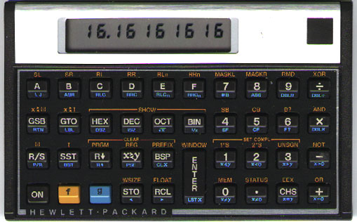
Before the TI-84 and its natural input system, there was the HP-16C. Well, it wasn’t the first of its kind, but it was the one people remembered.

There was a trend in the 70s and 80s to manufacture calculators that read input through something called Reverse Polish Notation. To understand, let’s take a quick detour, starting with something that you’re (I hope) more familiar with.

\[1 + (2 - (3 - 4) \times 5)\]

The above is a simple mathematical formula written in Infix Notation. Infix means that an operation $*$ on operands $a$ and $b$ is written with the operator located in-between (infix) the operands: $a * b$. It’s nice, but it has one huge problem: operator precedence (or order of operations). Call them PEMDAS or BODMAS, these rules you had to learn are school are… well, it’s obvious that they have to exist. There must be some specific order we read operations, otherwise it’d be ambiguous.

Actually… there’s another way. Try reading the above formula left-to-right, remembering each bit that is not useful yet (like the 1, that’s not really used until we know the value of the parentheses on the right). Then, keep track of each operation you perform. I know that it’s not how you would usually read it, but think of how you would explain a computer how to do it.

Doing the above, you get something like this:

• $1$, for later
• $+$, for later
• parentheses
  • $2$, for later
  • $-$, for later
  • parentheses
    • $3$, for later
    • $-$, for later
    • $4$
    • → nothing left, we get $3 - 4= -1$
  • $\times$, for later
  • $5$
  • → nothing left, we get $-1 \times 5 = -5$
  • → we still had that $2$ from earlier, we get $2 - -5 = 7$
• → nothing left, we get $1 + 7 = 8$

Admittedly, it’s quite convoluted. It’s almost like we’re trying to remember things, in order, with the most recently added items being used first…

We could try modeling the above a bit differently. Let’s say that instead of using operators ($+$, $-$, $\times$), we want to use functions (add, sub, mul). Let’s then rewrite the formula as a series of functions calls:

// 1 + (2 - (3 - 4) * 5)
add(1, sub(2, mul(sub(3, 4), 5)))

It’s readable, but there’s a lot of clutter because of all the required punctuation. But since we’re working with a really basic language where the only things are function calls and numbers, we can get rid of some of that code without making it ambiguous.

First, we can see that commas aren’t really useful. We know where a function name ends, and where a number begins:

add(1 sub(2 mul(sub(3 4) 5)))

Going further, we know in advance that each function takes two operands, so writing add 1 sub 2 3 wouldn’t be ambiguous: we know that 2 3 is a sequence of two numbers, that comes right after sub so it must be its parameters, and sub 2 3 is thus a function call. The same goes for the rest of the formula, add 1 sub 2 3 is not ambiguous when read that way. We can rewrite our bigger formula like this:

add 1 sub 2 mul sub 3 4 5

Since we’re doing math anyway, we might as well go back to the proper symbols:

+ 1 - 2 * - 3 4 5

Friends, what we have invented here is called the Prefix Notation. Prefix, because you write the operation before the operands (remember, Infix was when the operation is in-between). Though, it’s commonly known under another name: Polish Notation (because its inventor was Polish).

It’s the lesser known twin of the Postfix Notation (operation goes after the operands), commonly called Reverse Polish Notation (RPN) using which the formula would be written:

1 2 3 4 - 5 * - +

Of course, you may find those harder to read than our usual infix notation — which makes sense! You’ve been using infix all your life, your brain is wired to detect patterns in formulas written with the operator between its operands.

However, these notations have two huge advantages over infix:

• they don’t require parentheses or precedence rules
• they’re really easy to parse and evaluate

Both are actually two sides of the same coin: infix notation inherently needing artificial rules and parentheses to enforce evaluation order is precisely what makes it hard to parse. Parsing infix notation requires… writing a full-blown parser, or using magic like the shunting yard algorithm to convert it to RPN.

Here’s how simple an RPN evaluator can be:

import operator
operators = { "+": operator.add, "-": operator.sub, "*": operator.mul }

expr = "1 2 3 4 - 5 * - +"

items = expr.split() # cut into ["1", "2", ...]
stack = []
for item in items:
	if op := operators.get(item):
    	y = stack.pop()
        x = stack.pop()
        stack.append(op(x, y))
    else:
    	stack.append(int(item))
print("Result:", stack.pop())

There it is! A stack!

Evaluating an RPN formula pretty much comes down to making a simple stack machine. The formula then becomes some kind of simple machine language, where numbers are pushed on top of the stack and operators pop two numbers from the stack and push their result back.

And that simple language is what the HP-16C, and a slew of other handheld calculators released in the same era, spoke and understood. To type a formula, you’d enter each number, operator, keyword, and it would evaluate it, using a stack.

Keyword?

Well… we have three integer operations already; we might as well make this a full-fledged programming language. Say, let’s add the following:

• . pops from the stack and prints the value
• ! pops a name and a value from the stack, and assigns the value to the variable with that name
• @ pops a name from the stack and pushes back the value of the variable with that name
• dup duplicates the item at the top of the stack (in other words, pops a value and pushes it back twice)

Here are a few programs in our language:

• 5 3 + → 8
• 5 dup * → 25
• 1 2 dup * + dup + dup * hundred ! 2 hundred @ * → ?!

Yeah, that last one’s a bit contrived. Here’s a tabulated version, with the content of the stack at each step:

Code	Stack afterwards			Variables
1	1
2	1	2
dup	1	2	2
*	1	4
+	5
dup	5	5
+	10
dup	10	10
*	100
hundred	100	hundred
!				hundred = 100
2	2			hundred = 100
hundred	2	hundred		hundred = 100
@	2	100		hundred = 100
*	200			hundred = 100

As you can see, even with such a simple language and such a simple evaluation mechanism (cf. the RPN evaluator), we can do interesting stuff.

As a matter of fact, the language we’re using here is not imaginary at all: it’s actually (a subset of) Forth. It was designed in 1970 and gained popularity at the time because of its size; you could fit the compiler, editor, shell in very limited space, compared to languages such as Fortran or ALGOL. It’s still used nowadays in some fields, but it’s always been pretty niche.

It’s not the only language to use an “unusual” notation:

• the Lisp family, specifically the S-expression notation, uses prefix (Polish) notation for everything, so you get things like (+ 1 (- 2 (* (- 3 4) 5)))
• PostScript, like Forth, uses postfix (RPN) notation

However, the Lisp family is not really commonly used anymore (hi Clojure friends!) and PostScript is usually software-generated.

---

For a Few Stacks More

Ever heard of macros?

Do you ever think to yourself, while writing code, “man, this code would be so much clearer if it were written for a stack machine”? Me neither.

However, back in August, this Tweet popped in my feed:

i had a fucking disgusting idea today 🦀 pic.twitter.com/dU0eEFn8QA

— naomi (forgetful functor) (@fixedpointfae) August 19, 2022

Our old friend Forth, as a Rust macro.

A marvel of engineering, but it used stuff like HashMaps, so it wasn’t truly compile-time. So, naturally, I opened up a Playground session and started blasting.

The goal, here, is to implement a Rust declarative macro that reads Forth code and evaluates to the value of that bit of code. There are a few things to unpack here:

• Rust macro: takes a Rust syntax tree and outputs another Rust syntax tree. Basically, you can process code at compile time. Like C macros, but advanced.
• Rust declarative macro: a Rust macro that you can define directly in a Rust source file, using a special syntax that allows declaring patterns to match on, and complex substitutions rules. They can’t do anything macros can do, but they’re still quite powerful.
• Evaluate Forth code: run the Forth program on an imaginary Forth computer. The result is what’s left on top of the stack afterwards. A well-formed program, for our purpose, can leave any number of items on the stack; if the stack is empty, we’ll consider that the program returned nothing (in Rust terms, ()).

Here’s a relatively simple declarative macro that reproduces the built-in try! macro (ancestor of the ? operator):

/// "try_" macro. 
/// Evaluates the operand, then gives its value if it's Ok(...)
/// or returns Err(err) otherwise.
macro_rules! try_ {
	// Expects an expression
    ($expr:expr) => {
    	// The try_!(...) call is replaced by the "match" block below:
        match $expr {
            Ok(val) => val,
            Err(err) => {
                return Err(err);
            }
        }
    };
}

fn main() -> Result<(), impl Error> {
	let num: i32 = try_!("123".parse()); // equivalent to = "123".parse()?;
	let num: i32 = try_!("abc".parse());
    Ok(())
}

Declarative macros can take all sorts of parameters. Here, I’m specifying expr, because I expect try_! to be called with an expression, but I could want to process a statement, an identifier, a code block, etc. Everything a Rust file can contain, a declarative macro can process. A bit of code can be matched by multiple parameter types — for example, foo could be matched by:

• expr: an expression containing the binding name foo
• stmt: a statement fetching the value of foo and doing nothing with it
• ident: the identifier foo
• path: the path foo (a path is something like std::foo::bar)
• pat: the pattern foo (which matches everything)
• meta: the meta item foo (meta items are what comes in #[...])

foo + bar could be matched by:

• expr: an addition
• stmt: a statement computing an addition and doing nothing with it
• ty: a trait constraint (think where T: foo + bar)

You can do all sort of things with these types, but there’s a special one that I haven’t mentioned yet, and that would match all of the above examples — actually, it would match pretty much anything: tt.

It stands for “token tree”, and in layman’s terms (I’m really oversimplifying here), it basically means “whatever”. There are some limitations: you can’t write something like my_macro!( ) ) and expect tt to match the single parenthesis in the middle, since the whole isn’t valid Rust code. But apart from such edge cases, you’re pretty much unstoppable.

So, we wanted to evaluate Forth using a declarative macro. Intuitively, it should look like our RPN evaluator from before, but with a few more keywords. There’s a problem, though: we can’t have state! In our evaluator, we’re storing and modifying a list (the stack), and iterating, and here, we have neither state nor iteration. We have… substitution rules. Is it a dead end?

Remember earlier, when we talked about recursion and iteration and how they’re related. Well, the same way our count_files function could be written both recursively and iteratively, though by using, in essence, the same algorithm underneath, we can rewrite our RPN evaluator to use recursion!

import operator
operators = { "+": operator.add, "-": operator.sub, "*": operator.mul }

expr = "1 2 3 4 - 5 * - +"

items = expr.split() # cut into ["1", "2", ...]

def rpn(tokens, stack):
	if not tokens:
		return stack[0]
	item, *next_tokens = tokens
	if op := operators.get(item):
    	y, x, *rest = stack
        return rpn(next_tokens, [op(x, y), *rest])
    else:
    	return rpn(next_tokens, [int(item), *stack])

print(rpn(items, []))

Note that it looks like I’m mutating things here and modifying state, but if you look closely, I’m only declaring local variables in my function. The token list and the stack are never modified, I’m simply calling the function recursively with copies of those lists or sublists of them.

Now, we only have to write the above as macros. The nice part is that the items = expr.split() bit is already handled by the Rust parser! 1 2 3 ... is read as a token tree containing multiple tokens, one after the other. And macros allow consuming a token tree one token at a time. Here’s the result:

macro_rules! rpn {
	// +/-/*, pop two numbers, apply operator, push result
	(@eval [$y:expr, $x:expr, $($stack:tt)*] + $($rest:tt)*) => {
		rpn!(@eval [($x + $y), $($stack)*] $($rest)*)
	};

	(@eval [$y:expr, $x:expr, $($stack:tt)*] - $($rest:tt)*) => {
		rpn!(@eval [($x - $y), $($stack)*] $($rest)*)
	};

	(@eval [$y:expr, $x:expr, $($stack:tt)*] * $($rest:tt)*) => {
		rpn!(@eval [($x * $y), $($stack)*] $($rest)*)
	};

	// number, push to stack
	(@eval [$($stack:tt)*] $num:literal $($rest:tt)*) => {
		rpn!(@eval [$num, $($stack)*] $($rest)*)
	};

	// end of program, return top of stack
	(@eval [$top:expr, $($stack:tt)*] ) => {
		$top
	};

	// or, if stack empty, just return void
	(@eval [] ) => {
		()
	};

	// entry point
	($($tokens:tt)*) => {
		rpn!(@eval [] $($tokens)*)
	};
}

fn main() {
	println!("{}", rpn!(1 2 3 4 - 5 * - +));
}

The token list and the stack are passed as arguments to recursive calls of the macro. Rust allows using @ to write special tokens that can’t be written outside of a macro definition, so we can restrict the possible entry points to only the last macro rule (so others can only be called from inside the macro itself).

Here’s how the macro is expanded, step-by-step:

Code	Matched rule
1 2 3 4 - 5 * - +	$($tokens:tt)*
@eval [] 1 2 3 4 - 5 * - +	@eval [$($stack:tt)*] $num:literal $($rest:tt)*
@eval [1,] 2 3 4 - 5 * - +	@eval [$($stack:tt)*] $num:literal $($rest:tt)*
@eval [1,2,] 3 4 - 5 * - +	@eval [$($stack:tt)*] $num:literal $($rest:tt)*
@eval [1,2,3,] 4 - 5 * - +	@eval [$($stack:tt)*] $num:literal $($rest:tt)*
@eval [1,2,3,4,] - 5 * - +	@eval [$y:expr, $x:expr, $($stack:tt)*] - $($rest:tt)*
@eval [1,2,-1,] 5 * - +	@eval [$($stack:tt)*] $num:literal $($rest:tt)*
@eval [1,2,-1,5,] * - +	@eval [$y:expr, $x:expr, $($stack:tt)*] * $($rest:tt)*
@eval [1,2,-5,] - +	@eval [$y:expr, $x:expr, $($stack:tt)*] - $($rest:tt)*
@eval [1,7,] +	@eval [$y:expr, $x:expr, $($stack:tt)*] + $($rest:tt)*
@eval [8,]	@eval [$top:expr, $($stack:tt)*]
end of recursion, return 8

There! We can now evaluate RPN expressions, at compile time. No runtime cost whatsoever. If it’s invalid, it won’t compile. Ain’t that great?

Well, we wanted to make a Forth evaluator, this only supports a 3-operation RPN. That’s true, however, implementing other Forth operations is not difficult using our current architecture. We can implement variables by adding these 3 rules:

// variable name, push to stack
(@eval [$($e:tt)*] $var:ident $($x:tt)*) => {
	rpn!(@eval [$var, $($e)*] $($x)*)
};

// @, just evaluate the variable with the name
(@eval [$var:ident, $($e:tt)*] @ $($x:tt)*) => {
	rpn!(@eval [$var, $($e)*] $($x)*)
};

// !, create a variable
(@eval [$var:ident, $val:expr, $($e:tt)*] ! $($x:tt)*) => {
	{
		let $var = $val;
		rpn!(@eval [$($e)*] $($x)*)
	}
};

The end result is macro-forth, and it looks like this:

fn main() {
    const TWO: i32 = forth!(5 3 -);
    forth!(
        TWO . // 2
    );

    const HUNDRED: i8 = forth!(
        1 2 dup * + dup + // 10
        dup * // 100
        hundred !
        3 dup swap drop drop
        hundred @
    );

    forth!(
        HUNDRED @ dup . // 100
        50 > if "bigger" else "smaller" then . // bigger
    );
}

Generally, a macro such as this one that uses tt to “match anything” and consume token after token is called a tt-muncher, and it’s a very common pattern in Rust declarative macros, simply because it’s so powerful. As we’ve seen, anything (“any algorithm”) can be implemented using recursion, so it’s possible to do amazing stuff with this technique.

---

Parting words

Phew. This is my longest blog post yet. Both the macro one and the CPU one were about 4k words long, this one is at almost 7k and there are still things I wanted to put in that didn’t make the cut because it was really getting too long. I really hope you found it interesting, if not, I’ll do my best to make a better one next time!

As always, thank you for reading, if you have anything to say (positive or negative!) there’s a comment box below.

This blog post is provided “as is”, without warranty of any kind, though I do my best to write as few dumb things as possible.